Right-Sizing Serverless Compute Memory and Concurrency Settings

Right-sizing serverless compute means recognizing that memory, CPU allocation, concurrency, and cold-start behavior form a single coupled system, and tuning any one of them in isolation tends to produce a worse outcome. Most teams never make this discovery on purpose. A function gets deployed with whatever memory value the console suggested or a teammate copied from another project, it passes its tests, it ships, and nobody looks at it again until a bill lands that is three times larger than expected or a dashboard shows p99 latency climbing during a traffic spike. By then the function has been running in production for months, and the fix usually starts with someone bumping the memory slider up and hoping, the same mental model that caused the problem. Memory on a serverless platform is not just a capacity setting that keeps a function from running out of RAM. It also sets CPU allocation and the billing rate per second, and those three effects interact with each other and with concurrency in ways a single number can never represent.

Memory, CPU, and duration interaction on a real platform

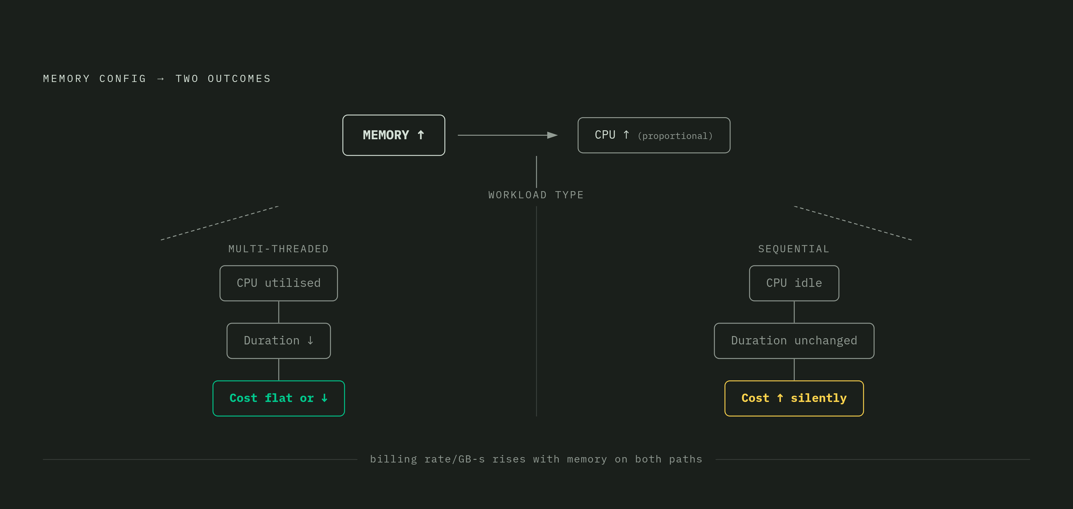
AWS Lambda ties CPU allocation directly to configured memory: pick a higher memory tier and the function gets proportionally more vCPU power along with it. That sounds like a straightforward trade, more memory for more speed, but it runs into a wall the moment the code itself cannot use the extra CPU. Sequential code only ever runs on one vCPU no matter how many are sitting available, so a single-threaded handler given four times the memory still executes at the same speed while Lambda bills at the higher rate for the entire duration. The extra compute sits there unused, like paying for a four-lane highway to drive a single car down it.

The benefit shows up only when the workload can actually spread its work across multiple cores. AWS has published benchmarks of multi-threaded Rust functions on Lambda that make this concrete: running on ARM64 with six parallel workers at the maximum memory setting produced a meaningful speedup, and the gap between median and tail latency stayed close to zero. That is what memory tuning looks like when the code is built to exploit the CPU it's given. A sequential function handed the same memory increase sees no change in duration at all, just a proportional rise in cost, because Lambda bills on GB-seconds: configured memory multiplied by billed duration. Billing uses the configured memory value, not the function's actual peak memory consumption, so if you size a function well above what it needs, you keep paying the higher rate for every millisecond it runs, even if it never touches that capacity.

This same coupling appears outside of general-purpose compute, in managed inference platforms. Amazon SageMaker Serverless Inference auto-assigns compute resources in direct proportion to the memory a developer selects. The memory-to-CPU link is therefore not a Lambda quirk. It is a general pattern in how these platforms allocate resources: scale the memory, and the compute scales with it, not independently.

Processor architecture adds a second, separate lever on top of all this. ARM64 instances on Lambda cost less per GB-second than x86, and most Node.js and Python functions can run on ARM64 without any code changes. You get that cost reduction through a single configuration switch, and it works no matter what memory value you choose. Skipping it is leaving money on the table for no reason.

Profiling before tuning: segmenting invocations so the data is actionable

If you average across a function's invocations, the number you get describes nothing real. A function that serves both a lightweight health check and an occasional 50 MB file transformation will report an average duration that matches neither workload, and tuning against that average will help one case while quietly hurting the other. Useful profiling starts with segmentation, breaking invocations apart before any metric gets interpreted.

You should segment by function version and by trigger type, because an API Gateway request, an SQS message, and a scheduled EventBridge trigger behave on different timelines and tolerate different latencies. Segment by payload size, since small and large payloads are effectively different workloads wearing the same function name. Separate cold starts from warm starts, because blending them obscures how much of a function's tail latency comes from initialization versus the handler logic itself. Separate successes from errors and timeouts, since a function that times out has still burned its full configured duration and may trigger a retry that burns it again. If a function serves multiple tenants or operation types, you should segment by that too, because heterogeneous work hiding under one function name will skew every aggregate metric you collect against it.

Within each segment, a specific set of metrics earns its place on a dashboard: billed duration tracked separately from handler duration, maximum memory used as a warning signal when it creeps close to the configured ceiling, and initialization duration isolated wherever the platform exposes it, since that number is the cold-start contribution on its own. Low peak memory usage is often read as proof that memory can be cut, but it says nothing about whether CPU can be reduced too, since memory and CPU are governed by the same dial for different reasons. Add invocation count, error rate, timeout rate, and throttle rate. For queue and stream triggers, add event age, queue depth, and retry count, since those triggers are optimizing for drain time. Downstream behavior matters just as much: a function tuned to run faster that then overwhelms a database connection pool has not solved a problem, it has relocated one.

The metric that ties all of this together is cost per successful invocation. A function that runs fast but fails a meaningful fraction of the time has a cost profile that looks nothing like its raw duration numbers suggest, because every failed invocation still consumes billed duration and may trigger a retry that consumes it again. Cost per successful invocation is the number that exposes this, and it is the number most tuning efforts never calculate.

Synthetic benchmarks cannot substitute for this kind of profiling. A loop of arithmetic run in isolation tells a developer nothing about network round trips, serialization overhead, decompression, or library initialization time, and those are frequently where the real cost and latency live. AWS Lambda Power Tuning, an open-source tool that AWS itself points developers toward, automates running representative payloads against multiple memory configurations within an account and compares the results. It is the right instrument for the benchmark sweep that follows, but it is only as good as the segmented, production-shaped data fed into it.

Benchmarking the memory curve to find the cost-performance optimum

The right memory setting for a function is a number found through measurement, not calculated from a spec sheet. To find it, you run representative payloads at several memory tiers and compare cost per successful invocation at each tier, not just the per-millisecond billing rate.

A proper sweep records, at every memory setting tested, the p95 duration, the error rate, and the cost per successful invocation. The payloads and SDK calls used in that sweep need to look like production traffic, not a synthetic arithmetic loop, because network calls, serialization, and dependency initialization are often the dominant cost and a synthetic benchmark hides all three. AWS Lambda Power Tuning automates this sweep across memory configurations within an account, which turns what used to be a manual, error-prone process into something that can run repeatedly as code and traffic patterns change.

The configuration to choose is the one that meets latency, error, and timeout targets with some headroom to spare, not the cheapest point on the curve in isolation. A function running right up against its memory ceiling is a risk no matter how good its cost-per-invocation number looks, because the next slightly larger payload will push it over. Under-provisioning stretches duration and degrades tail latency; over-provisioning pays for CPU and memory the function never touches. The curve between those two failure modes has a minimum, and that minimum can only be located by measuring both sides of it.

AI inference workloads carry a hard floor on top of this curve. Amazon SageMaker Serverless Inference requires memory to be at least as large as the model held in memory, with an overall minimum of 1 GB and a maximum of 6 GB. That floor is set by model size, not by the latency-cost tradeoff, so the benchmark sweep for an inference endpoint only has room to operate above wherever that floor lands.

Once a sweep identifies a candidate memory setting, publish it as a new version and route a controlled slice of traffic to it, whether through an alias weight or a partitioned event stream, before committing the whole fleet to it. Test that candidate under both steady-state and peak load, because a configuration that looks optimal on average traffic can behave very differently once the queue backs up. And a memory change rarely stops at memory: if the new setting changes a function's duration, it has also changed how much concurrency that function needs to handle the same arrival rate. That's the next lever, and it does not move independently of the one just adjusted.

Deriving concurrency requirements from arrival rate and duration

Concurrency is not a number to pick by instinct. For synchronous workloads it can be derived directly: concurrency is approximately requests per second multiplied by average duration in seconds. That formula is also where the coupling with memory tuning becomes unavoidable. If a memory change cuts a function's duration in half, it also cuts the concurrency needed to serve the same arrival rate in half. Most tuning guides treat memory and concurrency as two separate dials to be set independently, but a change to one changes the required value of the other every time.

If you plan for real traffic, you plan against a distribution, not an average. If you plan for bursts, you need peak-interval arrival data, because a traffic spike lasting ninety seconds can saturate a function sized only for its daily average arrival rate. Account-level concurrency limits on Lambda are a hard ceiling: once that ceiling is hit, new invocations get throttled with 429 errors. There is no graceful slowdown built in, only a wall. Reserved concurrency assigned to one function also narrows the headroom available to every other function in the account, even while that reserved function sits idle, so reserving concurrency for one workload has a cost measured in what it takes away from the rest.

But with queue and stream triggers, the objective changes entirely, from request latency to drain time or event age. Pushing concurrency up drains a backlog faster, but it can also overwhelm whatever sits downstream: a database, an API with its own rate limits, a NAT gateway, a connection pool with a fixed ceiling. You can set a reserved or trigger-level concurrency cap as a safety valve here, but you need to test that cap's retry behavior directly, because aggressive retries against an already-constrained downstream system make the shortage worse and stretch the backlog.

The three concurrency modes on Lambda carry distinct cost and behavior tradeoffs, and people confuse two of them often enough that the difference needs stating precisely. Reserved concurrency caps and sets aside capacity for a specific function, but it does not pre-initialize any environments, so a reserved function can still hit a cold start. Provisioned concurrency pre-initializes a set number of warm environments and charges continuously for them regardless of how much traffic actually arrives, making it a reserved-compute billing model running inside a serverless platform. On-demand concurrency is the default, and it scales freely within account limits at no extra charge, but it still hits the same hard throttling ceiling described above.

This derivation logic holds across platforms even though the specific knobs differ. Azure Functions distinguishes fixed and dynamic per-instance concurrency across its plans, and Flex Consumption adds deterministic per-instance concurrency controls, including configurable HTTP trigger concurrency per instance, that the legacy Consumption plan does not expose in the same form. Cloud Run also exposes its own minimum and maximum instance counts alongside per-instance concurrency settings. The arithmetic connecting arrival rate, duration, and concurrency is the same wherever it is applied; only the dials used to act on it change, and each platform's documentation confirms how.

Cold starts as the fourth variable

Cold-start latency is not a fixed tax a platform charges on every function equally. It moves with memory setting, package size, runtime choice, and how much initialization code runs outside the handler, and it interacts directly with whatever concurrency model has already been chosen.

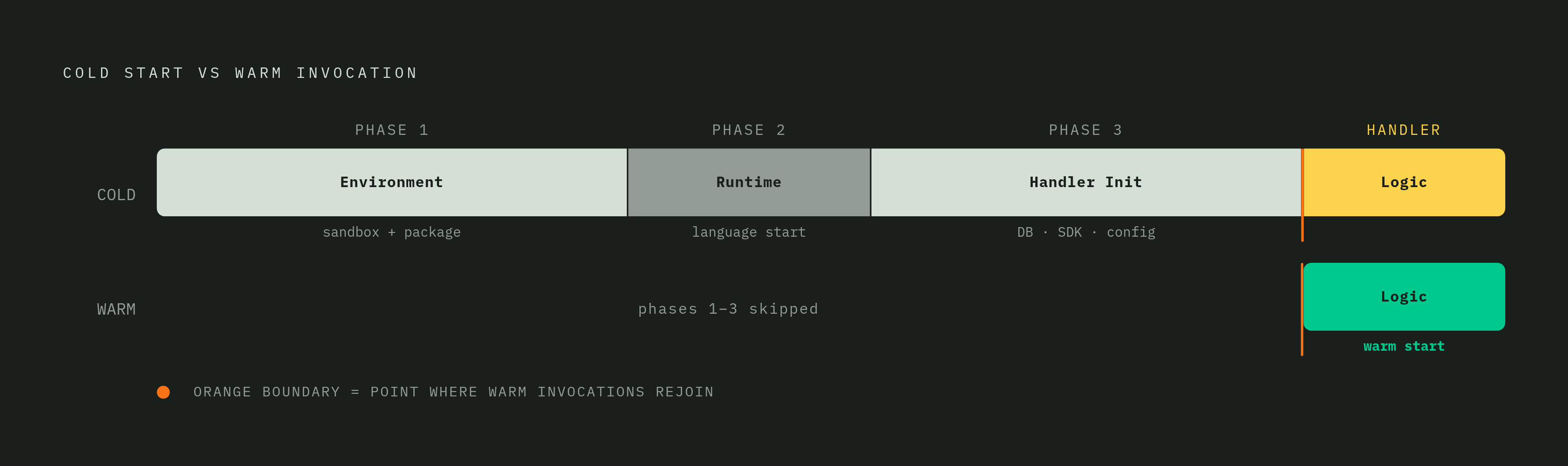
A cold start is three phases stacked together. Environment preparation downloads the deployment package and provisions the execution sandbox. Runtime initialization starts the language runtime itself. Handler initialization runs whatever global-scope code sits outside the handler function, so it opens database connections, constructs SDK clients, and loads configuration there. Only that last category, the handler's own work, runs on a warm invocation. All three phases run every time a cold start occurs, so a cold start costs meaningfully more than a warm invocation even before the handler logic executes a single line.

How often cold starts happen is itself a function of the concurrency decisions made earlier. When traffic exceeds the number of already-warm execution environments, new ones get created, and the rate at which that happens depends on arrival rate, duration, and how many environments are already provisioned or warm. The four variables are one system viewed from four angles, not four separate projects.

Each mitigation for cold starts carries its own cost. Moving reusable initialization, SDK clients and connection pools, outside the handler lets a function take advantage of execution context reuse on subsequent invocations, though that reuse is probabilistic rather than guaranteed, so it helps without eliminating the problem. Trimming unused dependencies and lazy-loading rarely used code paths shrinks package size and initialization time at no cost, though the upside shrinks once a function's dependencies are already lean. Provisioned concurrency removes cold starts entirely for however many environments it covers, but it turns those environments into always-on compute billed continuously, so the billing model shifts away from serverless economics for that portion of capacity. Scheduled warm-up pings exist as a workaround, but they carry fragile timing guarantees and offer no cost advantage over provisioned concurrency at any meaningful scale.

Provisioned concurrency earns its cost when it is sized to cover typical peak demand plus a buffer, not when it is sized to eliminate every cold start at the absolute ceiling of traffic a function might someday see. On-demand concurrency can absorb the rare burst while provisioned capacity handles the predictable load band underneath it. SageMaker Serverless Inference with Provisioned Concurrency follows the identical pattern: provisioned capacity keeps an endpoint warm through predictable bursts, billed by the millisecond for capacity used plus a separate provisioned concurrency charge on top. If your test suite only exercises already-warm environments, warm-traffic testing alone will never catch any of this, since it has nothing to say about cold-start contribution to tail latency. That number has to be measured on its own, using the initialization-duration metric isolated during profiling, the same metric the profiling framework called for at the start of this process.